How the (Econometric) Sausage is Made

Panel data has become quite abundant. As a result, fixed effects models have become prevalent in applied research. But, this week I handled a paper at one of the journals for which I am on the editorial board and was reminded of a mistake that I have seen all too frequently over the years. Most researchers are probably aware of the issue I am highlighting, but indulge me. In a cross-sectional regression model, we have y_i = a + b*x_i + e_i OLS is unbiased if x is exogenous , which requires that Cov(x_i,e_i) = 0. In other words, the covariates need to be uncorrelated with the error term from the same time period. In contrast, in a panel regression model with individual effects, we have y_it = a_i + b*x_it + e_it If we wish to allow for the possibility that Cov(a_i,x_it) differs from zero, then a_i is a "fixed" effect instead of a "random" effect. To understand what we need to assume to obtain unbiased estimates of b, we need to understand how the model i

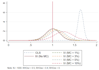
Today I am going to take the opportunity to plug a short paper I wrote a few years ago. I remember a senior colleague telling me when I was an AP that as you age, you become much more concerned about your legacy. You write papers that you want to write, rather than worrying about tenure or other sources of external validation. The paper I am going plug falls squarely in this realm. I wrote it because I wanted to, regardless of what became of it. As you can tell from my first few posts in this blog, I enjoy thinking about measurement error and endogeneity more generally. As both problems are very common in applied work, starting many years ago (yes, I am old) ... I was increasingly coming across applied papers that confronted both issues. Specifically, papers that are interested in the causal effect of a covariate of interest on some outcome, but must confront the dual problems of said covariate being measured with error and being potentially endogenous (due to omitted unobserved

The issue here is to consider a very simple model, Y = a + b*D + e, where D is a binary variable and b is the coeff of interest. Suppose D is endogenous, but we have a valid instrument, z. IV is consistent and should do well in large samples if z is strong. But what if D is also measured with error? I.e., what if the true model is Y = a + bD* + e, where D* is the true D, but we only observe D (D not equal D* for some i)? That valid instrument, z, we had? Now, it's not quite as useful. Why? Because ME in a binary var canNOT be classical. When D*=0, the ME can only be 0 or 1. When D*=1, the ME can only be 0 or -1. Thus, the ME is necessary neg. corr. with D*. Since the IV, z, is correlated with D*, it is almost assuredly also correlated with the ME and thus invalid. A very good reference is Black et al. (2000). Note, this argument applies to any bounded variable; D* need not be binary. E.g., if D* represents a percentage, then it is bounded on the unit interval. If

Applied papers that rely on instrumental variables are often focused solely on a single parameter of interest. This parameter is the coefficient on an endogenous variable. Using an IV for this variable, one obtains the IV estimate of this coefficient. But what about all those other "exogenous" vars in the model? Usually the coefficient estimates are ignored because they are not "of interest." What if one of those exogenous control variable is really endogenous as well? The typical response: "I don't care about that coefficient, so it doesn't matter." But does it matter? Um, perhaps yes! Let's say the true model is Y=a+b1*x1+b2*x2+e and both x1 and x2 are endogenous. You only care about b1. You have an IV for x1, call it z. For z to be valid, we know it must be correlated with x1 and uncorrelated with e. But ... it also needs to be (in all likelihood) uncorrelated with x2! If your IV is correlated with an endogenous regressor inco

Today I'm getting into the weeds a bit about how "finicky" (as I describe it) the IV estimator is. Before describing some of the downside to IV, I think it is worth saying that I think IV gets a very bad wrap. It's a great solution to a very common problem ... under the right assumptions. If those assumptions hold, don't be ashamed to use it. Clearly, that's a big "if" and, as they say, therein lies the rub. So, one thing that makes IV "finicky" is that it a consistent estimator, but it is not unbiased. I think most people know this (but I do see references to IV producing "unbiased causal effects" far too often). Perhaps less well known is that in exactly identified models t he expectation of the estimator does not exist! For those who perhaps don't recall, consistency is an asymptotic property based on taking plims. Bias is a finite sample property based on expectations. So, in finite samples (and I have yet to see an

Applied economists are often interested in models where a covariate enters in quadratic form. For instance, the Kuznets curve and Environmental Kuznets curve posit inverted-U relationships between inequality and pollution, respectively, and income. The Mincer wage equation includes a quadratic for age or experience. Many other theoretical models give rise to non-linear effects of a covariate on outcomes. How classical measurement error impacts the estimates is not given a lot of thought. But ... it should be. Suppose one estimates a quadratic model y = a + b1*x + b2*x^2 + e that satisfies all the assumptions of the CLRM except x suffers from classical measurement error. Griliches & Ringstad (1970) show that (under normality) the OLS estimates of b1 and b2 both suffer from attenuation bias. However, the bias of b2 is more severe; the plim for b2 is b2 times the squared reliability ratio. Since the reliability ratio (the ratio of the variance of the true x to the variance of

Classical ME results in attenuation bias. We all (hopefully) know that. But ... The bias depends on the ratio of the variance of the measurement error, μ, to the variance of the observed X not explained by other covariates. Formally, this is shown below where the degree of the attenuation bias depends on the R2 from a regression of X on the remaining covariates in the model. The implication is that even "small" measurement error (as captured by the variance of μ) can be enormously consequential in multiple regression. It is not sufficient IMHO to dismiss measurement error simply because you believe it to be "small." On top of that, ignoring measurement error in a covariate because it is not the "regressor of interest" is a common, but costly, mistake. Measurement error in a control variable in your regression model will (in all likelihood) bias your coefficient of interest if the regressor of interest is correlated with the mismeasured regresso

I am somewhat reluctantly starting this blog on econometric stuff that applied people will hopefully find useful. I am wary to do so because I do not consider myself to be an econometrician; I am an applied econometrician. As such, I suffer from a bit of imposter syndrome in creating a blog on econometric topics. That said, my goal is to make applied types aware of some issues - in as nontechnical way as possible (as I said, I am not an econometrician) - that arise in typical applied (micro) research. The issues I find fascinating are the subtle parts of econometrics that individuals either may not have learned or may have forgotten. By diving a bit into how various econometric methods work in practice, we hopefully will all better understand how the econometric sausage is made. Perhaps ignorance is bliss, but as economists we tend to relish in the dismal. I am fortunate to teach econometrics at SMU and think all empirical types should teach econometrics. It's amazing what you