How the (Econometric) Sausage is Made

In one of the greatest movies ever made, Miracle Max says: "Turns out your friend here is only MOSTLY dead. See, mostly dead is still slightly alive." Well, there is a lesson to be learned. In econometrics, many parameters that one might consider to be unidentified are only MOSTLY unidentified. And, following Miracle Max's unassailable logic, mostly unidentified is still slightly identified.  Miracle Max continues to share his wisdom with us mere mortals when he says that with "ALL dead, there is only one thing you can do ... go through his pockets and look for loose change." With ALL unidentified, I suppose all we can do is thank our academy for a lovely run and turn off the lights on our way out.   But, what do we do when confronted with mostly unidentified parameters? Well, that's where partial identification -- played here by Miracle Manski -- enters the scene. Partial identification econometric techniques existed before Manski, but ...

Structural breaks. The stuff of time series. You cannot be a time series econometrician and not be well-versed in the importance of allowing for, testing for, and dealing with structural breaks (or so I am told). However, surely there is something to to be learned from this literature that applied microeconometricians can utilize, no? Spoiler: Yes, there is! Applied microeconometricians, who may be unaware of the tremendous advances in the literature on structural breaks, would be wise to take notice. While break dancing may not have advanced since last century and may have little to offer to today's generation, testing for structural breaks has advanced and has much to offer. To understand, let us review. A structural break refers to any change in the underlying data-generating process (DGP). Some fraction of the sample is drawn from one DGP; some other fraction is drawn from another DGP. Of course, there may be more than one structural break and, hence, more th...

If you think this post is about inflation of the macro variety, you have come to the wrong place! This is about inflation of the econometric (and typically micro) variety. When modeling discrete data -- count data or otherwise -- we often find that one value occurs much more frequently than the rest. Standard models for discrete outcomes (usually referred to as limited dependent variable models) do not fit the data well in such situations because they have some type of "smoothness" (implicitly) built in to the assumed data-generating process. This causes the estimated model to under-predict the frequently occurring outcome and over-predict other outcomes. To better fit the data in such situations, so-called "inflated" limited dependent variable models were created. As far as I know, early work in this area cites Cragg (1971) and Mullahy (1986). The literature started with count data models when zeros occurred with high frequency in the sample. This led t...

Binary choice models. Statistical models used to analyze the determinants of a binary outcome. Employed or not employed. Enrolled in school or not enrolled. Defaulted on a loan or not. WTO member or not. Democratic or not. And on and on. The analysis of binary outcomes is frequent and important in economics, political science, sociology, epidemiology, and others. So, we should strive to get it right. Getting it "right" has meant a lengthy debate - that has seemingly gone on  ad nau seam  - over the choice between a linear probability model (LPM) and a probit or logit model.  For those unaware, LPM is a fancy name for "I am going to use OLS even though the dependent variable is binary, but I want to feel special!"  Probit and logit, on the other hand, are estimated via maximum likelihood (the original ML).  Now that we have covered the basics, here is the twist. This is most definitely NOT another blog post on the relative merits of LPM and probit/l...

Panel data has become quite abundant. As a result, fixed effects models have become prevalent in applied research. But, this week I handled a paper at one of the journals for which I am on the editorial board and was reminded of a mistake that I have seen all too frequently over the years. Most researchers are probably aware of the issue I am highlighting, but indulge me. In a cross-sectional regression model, we have y_i = a + b*x_i + e_i OLS is unbiased if x is exogenous , which requires that Cov(x_i,e_i) = 0. In other words, the covariates need to be uncorrelated with the error term from the same time period. In contrast, in a panel regression model with individual effects, we have y_it = a_i + b*x_it + e_it If we wish to allow for the possibility that Cov(a_i,x_it) differs from zero, then a_i is a "fixed" effect instead of a "random" effect. To understand what we need to assume to obtain unbiased estimates of b, we need to understand how the model i...

Today I am going to take the opportunity to plug a short paper I wrote a few years ago. I remember a senior colleague telling me when I was an AP that as you age, you become much more concerned about your legacy. You write papers that you want to write, rather than worrying about tenure or other sources of external validation. The paper I am going plug falls squarely in this realm. I wrote it because I wanted to, regardless of what became of it. As you can tell from my first few posts in this blog, I enjoy thinking about measurement error and endogeneity more generally. As both problems are very common in applied work, starting many years ago (yes, I am old) ... I was increasingly coming across applied papers that confronted both issues. Specifically, papers that are interested in the causal effect of a covariate of interest on some outcome, but must confront the dual problems of said covariate being measured with error and being potentially endogenous (due to omitted unobserved ...

The issue here is to consider a very simple model, Y = a + b*D + e, where D is a binary variable and b is the coeff of interest. Suppose D is endogenous, but we have a valid instrument, z. IV is consistent and should do well in large samples if z is strong. But what if D is also measured with error? I.e., what if the true model is Y = a + bD* + e, where D* is the true D, but we only observe D (D not equal D* for some i)? That valid instrument, z, we had? Now, it's not quite as useful. Why? Because ME in a binary var canNOT be classical. When D*=0, the ME can only be 0 or 1. When D*=1, the ME can only be 0 or -1. Thus, the ME is necessary neg. corr. with D*. Since the IV, z, is correlated with D*, it is almost assuredly also correlated with the ME and thus invalid. A very good reference is Black et al. (2000). Note, this argument applies to any bounded variable; D* need not be binary. E.g., if D* represents a percentage, then it is bounded on the unit interval. If...

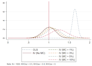
Applied papers that rely on instrumental variables are often focused solely on a single parameter of interest. This parameter is the coefficient on an endogenous variable. Using an IV for this variable, one obtains the IV estimate of this coefficient. But what about all those other "exogenous" vars in the model? Usually the coefficient estimates are ignored because they are not "of interest." What if one of those exogenous control variable is really endogenous as well? The typical response: "I don't care about that coefficient, so it doesn't matter." But does it matter? Um, perhaps yes! Let's say the true model is Y=a+b1*x1+b2*x2+e and both x1 and x2 are endogenous. You only care about b1. You have an IV for x1, call it z. For z to be valid, we know it must be correlated with x1 and uncorrelated with e. But ... it also needs to be (in all likelihood) uncorrelated with x2! If your IV is correlated with an endogenous regressor inco...