The Rollercoaster
Econometrics can be a wild ride. Trying to navigate the field as an applied researcher can be equally wild. But, sometimes it is exactly the wildness that makes the 'metrics work.
I was inspired (tasked?) by my good friend whom I have never met, Paul Hünermund, in a Twitter thread this week. He raised an old topic in econometrics that might be (vastly) underappreciated by applied researchers. The topic reminds me of a scene from the classic movie, Parenthood. All you struggling parents during the pandemic may be too young to have seen it. Now would be a good time to remedy that situation!
Oh geez, I just looked and it is from 1989. How old am I?
In the scene, Grandma relays the following bit of wisdom.
Grandma clearly appreciates the ups and downs, twists and turns, of the roller coaster. Its highly non-linear path. In contrast, the merry-go-round just stays flat. On a linear path.

In econometrics, as with roller coasters, the non-linearity can make all the difference. With roller coasters, non-linearity leads to fright and sickness and thrill. In econometrics, non-linearity can lead to identification, which is thrilling, but it can also lead to fright and sickness if we don't fully appreciate what is happening.

Many (most?) applied researchers have probably encountered the phrase, "identification through non-linearity". I still remember my advisor using it during my grad school classes and not understanding the concept. It is an important one to understand and appreciate.
Perhaps the most common situation in which the concept arises -- at least in empirical micro -- is the classic work in Heckman (1979) on sample selection. The setup is given by

In the problem, the regression model for y is assumed to satisfy all the usual assumptions of the Classical Linear Regression Model. Thus, if we had a random sample of {y,x}, then Ordinary Least Squares (OLS) is unbiased. However, if the outcome, y, is missing in a subset of our random sample (denoted by S=0), then the sample for which we actually observe {y,x}, given by S=1, may no longer be random.
The canonical example is when y is a measure of labor market wages for women and wages are unobserved for non-workers. In this case, S is equivalent to an indicator for working women.

We model the sample selection rule, S, using a probit model with covariates, z, where ρ represents the correlation between unobserved attributes affecting sample selection, u, and unobserved variables affecting the outcome, ε.
Heckman points out that while the OLS estimates of the regression model for y are unbiased in the absence of missing data on y, they will not be if ρ differs from zero. The bias arises because, while ε is a well-behaved error term in the population, it will not be in the sub-sample with S=1 unless ρ is zero (i.e., the data are missing at random).


where φ and Φ are the standard normal probability density function (PDF) and cumulative density function (CDF), respectively.
This leads to Heckman's two-step sample selection procedure
1. Estimate γ via probit model using the full sample. Obtain the IMR for each observation with S=1.
2. Estimate β via OLS, with the IMR included as an extra covariate, using the sample with S=1.
Taking the theme of roller coasters perhaps too literally, I have taken a long, winding road to get to the point.

The point is identification. Why does Heckman's approach work? The augmented model in Step 2 above is
y = xb + cIMR + w
where w is the well-behaved error term in the sample with S=1. However, while solving one problem (a misbehaving error term), we may have replaced it with another problem.

The new potential problem is multicollinearity between the original design matrix, x, and the IMR. Why? Well, if the functional form of the control function in Heckman's problem had not been the roller coaster (aka, non-linear), but instead had been the merry-go-round (aka, linear), then our estimating equation would have been

This is what is meant by identification through nonlinearity. When z=x, Heckman's solution only works because the control function is non-linear; were it linear, the model would be unidentified.
What's that you say? But it is non-linear?

The control function only has its particular functional form -- the IMR -- because of the assumption that the errors are bivariate normal, which we have no reason to believe. Moreover, the IMR isn't that non-linear. Thus, relying on technical identification is just like Grandma's roller coaster: thrilling, but frightening and scary!

There have been a number of studies published that discuss this and perform extensive simulations to evaluate performance in practice (Puhani 2000; Leung & Yu 2000; Bushway et al. 2007). Heckman's solution (as well as various semiparametric approaches that relax the bivariate normality assumption) can be quite volatile in practice when z and x are identical, or even highly correlated. So, while technically the model is identified through nonlinearity, one should not rely on it! Don't become another statistic!

At the risk of making this post much too long, let me tell you about three other examples in econometrics where identification is through non-linearity. One's cup of knowledge can never be too full!

First, Heckman's sample selection approach can easily to be extended to account for missing counterfactuals in the potential outcomes framework. The model setup is


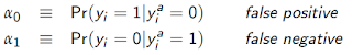
To understand the approach, assume that a logit is the correct model if the true (actual) outcome, y^a, is observed. However, the rates of false positives and negatives are given by

All of the parameters can be estimated via Maximum Likelihood using these probabilities. Seems a bit magical. Almost like a roller coaster!
Identification arises in the model because the logit probabilities for the true outcomes are non-linear functions of β. If one instead tried the same approach in a -- gasp! -- Linear Probability Model (LPM), one cannot separately identify the α's and the β's.


Third, Klein & Vella (2010) propose a solution to endogeneity when one lacks a valid instrumental variable (IV).


Bushway, S., B.D. Johnson, and L.A. Slocum (2007), "Is the Magic Still There? The Use of the Heckman Two-Step Correction for Selection Bias in Criminology," Journal of Quantitative Criminology, 23(2), 151-17
Hausman, J.A., J. Abrevaya, and F.M. Scott-Morton (1998), "Misclassification of the Dependent Variable in a Discrete-Response Setting," Journal of Econometrics, 87(2), 239-269
Heckman, J.J. (1979), "Sample Bias As A Specification Error," Econometrica, 47(1), 153-162
Hug, S. (2003), "Selection Bias in Comparative Research: The Case of Incomplete Data Sets,” Political Analysis, 11(3), 255-274
Hug, S. (2009), "The Effect of Misclassifications in Probit Models: Monte Carlo Simulations and Applications,” Political Analysis, 18(1), 78-102
Klein, R. and F. Vella (2010), "Estimating a Class of Triangular Simultaneous Equations Models Without Exclusion Restrictions," Journal of Econometrics, 154, 154-164
Leung, S.F. and S. Yu (2000),"Collinearity and Two-Step Estimation of Sample Selection Models: Problems, Origins, and Remedies," Computational Economics, 15(3), 173-199
Puhani, P. (2000), "The Heckman Correction for Sample Selection and Its Critique," Journal of Economic Surveys, 14(1), 53-68
I was inspired (tasked?) by my good friend whom I have never met, Paul Hünermund, in a Twitter thread this week. He raised an old topic in econometrics that might be (vastly) underappreciated by applied researchers. The topic reminds me of a scene from the classic movie, Parenthood. All you struggling parents during the pandemic may be too young to have seen it. Now would be a good time to remedy that situation!
Oh geez, I just looked and it is from 1989. How old am I?
In the scene, Grandma relays the following bit of wisdom.
Grandma : You know, when I was nineteen, Grandpa took me on a roller coaster.
Gil : Oh?
Grandma : Up, down, up, down. Oh, what a ride!
Gil : What a great story.
Grandma : I always wanted to go again. You know, it was just so interesting to me that a ride could make me so frightened, so scared, so sick, so excited, and so thrilled all together! Some didn't like it. They went on the merry-go-round. That just goes around. Nothing. I like the roller coaster. You get more out of it.
Grandma clearly appreciates the ups and downs, twists and turns, of the roller coaster. Its highly non-linear path. In contrast, the merry-go-round just stays flat. On a linear path.
In econometrics, as with roller coasters, the non-linearity can make all the difference. With roller coasters, non-linearity leads to fright and sickness and thrill. In econometrics, non-linearity can lead to identification, which is thrilling, but it can also lead to fright and sickness if we don't fully appreciate what is happening.
Many (most?) applied researchers have probably encountered the phrase, "identification through non-linearity". I still remember my advisor using it during my grad school classes and not understanding the concept. It is an important one to understand and appreciate.
Perhaps the most common situation in which the concept arises -- at least in empirical micro -- is the classic work in Heckman (1979) on sample selection. The setup is given by
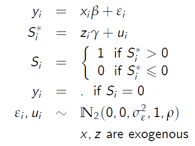
In the problem, the regression model for y is assumed to satisfy all the usual assumptions of the Classical Linear Regression Model. Thus, if we had a random sample of {y,x}, then Ordinary Least Squares (OLS) is unbiased. However, if the outcome, y, is missing in a subset of our random sample (denoted by S=0), then the sample for which we actually observe {y,x}, given by S=1, may no longer be random.
The canonical example is when y is a measure of labor market wages for women and wages are unobserved for non-workers. In this case, S is equivalent to an indicator for working women.
We model the sample selection rule, S, using a probit model with covariates, z, where ρ represents the correlation between unobserved attributes affecting sample selection, u, and unobserved variables affecting the outcome, ε.
Heckman points out that while the OLS estimates of the regression model for y are unbiased in the absence of missing data on y, they will not be if ρ differs from zero. The bias arises because, while ε is a well-behaved error term in the population, it will not be in the sub-sample with S=1 unless ρ is zero (i.e., the data are missing at random).
Fortunately, there is a solution. Given the probit structure for the sample selection process, we can restore the necessary properties of the error term in our regression model applied to the sub-sample with complete data by augmenting the model with a control function. A control function is a fancy term for anything extra we add to our model to make the error term well-behaved.
Stated differently, in situations where the error term is misbehaving, if we can pull out the naughty part and put it in the model itself (i.e., control for it), then what's left in the error term is now well-behaved. In the sample selection model considered by Heckman, the control function has a particular functional form, known as the Inverse Mills' Ratio (IMR).
This leads to Heckman's two-step sample selection procedure
1. Estimate γ via probit model using the full sample. Obtain the IMR for each observation with S=1.
2. Estimate β via OLS, with the IMR included as an extra covariate, using the sample with S=1.
Taking the theme of roller coasters perhaps too literally, I have taken a long, winding road to get to the point.
The point is identification. Why does Heckman's approach work? The augmented model in Step 2 above is
y = xb + cIMR + w
where w is the well-behaved error term in the sample with S=1. However, while solving one problem (a misbehaving error term), we may have replaced it with another problem.
The new potential problem is multicollinearity between the original design matrix, x, and the IMR. Why? Well, if the functional form of the control function in Heckman's problem had not been the roller coaster (aka, non-linear), but instead had been the merry-go-round (aka, linear), then our estimating equation would have been
y = xb + c(zg) + w
where g is the probit estimate of γ. Moreover, if z=x, implying identical covariates in the selection and outcome models, then our estimating equation would have been
y = xb + c(xg) + w.
And, this model is not identified due to perfect multicollinearity between the design matrix and the control function.
But, alas, the control function is not linear, it is the roller coaster. As such, even if z=x, the model reverts back to
y = xb + cIMR + w
where the IMR is a non-linear function of xg. Here, there is technically no problem of perfect multicollinearity because, although x and IMR are both functions of x, they are not linearly dependent. They are not riding the merry-go-round together. The non-linearity is technically sufficient for identification. As Grandma says, "I like the roller coaster."
This is what is meant by identification through nonlinearity. When z=x, Heckman's solution only works because the control function is non-linear; were it linear, the model would be unidentified.
What's that you say? But it is non-linear?
The control function only has its particular functional form -- the IMR -- because of the assumption that the errors are bivariate normal, which we have no reason to believe. Moreover, the IMR isn't that non-linear. Thus, relying on technical identification is just like Grandma's roller coaster: thrilling, but frightening and scary!
There have been a number of studies published that discuss this and perform extensive simulations to evaluate performance in practice (Puhani 2000; Leung & Yu 2000; Bushway et al. 2007). Heckman's solution (as well as various semiparametric approaches that relax the bivariate normality assumption) can be quite volatile in practice when z and x are identical, or even highly correlated. So, while technically the model is identified through nonlinearity, one should not rely on it! Don't become another statistic!
At the risk of making this post much too long, let me tell you about three other examples in econometrics where identification is through non-linearity. One's cup of knowledge can never be too full!
First, Heckman's sample selection approach can easily to be extended to account for missing counterfactuals in the potential outcomes framework. The model setup is

and the estimating equation becomes

which now includes two control functions. This approach technically addresses selection on unobserved variables without a traditional instrument as the non-linearity of the control functions circumvents perfect multicollinearity even when z=x.
Second, Hausman et al. (1998) propose a solution to misclassification of a binary outcome in a logit (or probit) model.
To understand the approach, assume that a logit is the correct model if the true (actual) outcome, y^a, is observed. However, the rates of false positives and negatives are given by

The authors then derive the probabilities for the observed outcome, y, given by

All of the parameters can be estimated via Maximum Likelihood using these probabilities. Seems a bit magical. Almost like a roller coaster!
Identification arises in the model because the logit probabilities for the true outcomes are non-linear functions of β. If one instead tried the same approach in a -- gasp! -- Linear Probability Model (LPM), one cannot separately identify the α's and the β's.

Third, Klein & Vella (2010) propose a solution to endogeneity when one lacks a valid instrumental variable (IV).
To understand their approach, one must first realize that the traditional IV estimator can be estimated using a control function approach. Estimation proceeds by
1. Estimate the first-stage using OLS. Obtain the first-stage residuals.
2. Estimate the second-stage using OLS, augmenting the set of covariates to include the first-stage residuals.
Thus, the second-stage becomes
The OLS estimate of β is identical to the IV estimate. However, for this to work, we need -- as in the Heckman models -- the control function not to be perfectly colinear with x. If the first-stage is
x = zg + u,
then the residuals are
u-hat = x - zg.
If z does not include an instrument, then u-hat will simply be a linear combination of x and perfect mulitcollinearity will result. An instrument allows us to stay on the merry-go-round.
Klein & Vella's solution is to foresake the instrument, and instead ride the roller coaster. They do so by providing a set of assumptions such that the control function in the second-stage, while still u-hat, now has an observation-specific coefficient, δ_i. Their strategy relies on, among other things, the first- and/or second-stage errors being heteroskedastic. Under their assumptions, the control function and its coefficient changes from
u-hat_i*δ
in the typical IV model to
u-hat_i*δ_i = u-hat_i*S_i*ρ,
where S_i is a non-linear function of the variances of the first- and second-stage errors.

Assuming a functional form for these variances, S_i along with the final model can be estimated. Importantly, even if the heteroskadasticity depends on only the x's included in the model, the model is identified because of the non-linearity of S_i.
The astute reader might also realize that this approach does not differ too much from simply using higher order terms and interactions of x as traditional instruments, which of course is also an example of identification through non-linearity. Nonetheless, the approach eschews 'traditional' instruments and prefers to ride the roller coaster!
Thanks for making it this far. It is now safe to ...
If you decide to stay on the metaphorical roller coaster, enjoy the ride! I'm sure it will be thrilling.
References
References
Bushway, S., B.D. Johnson, and L.A. Slocum (2007), "Is the Magic Still There? The Use of the Heckman Two-Step Correction for Selection Bias in Criminology," Journal of Quantitative Criminology, 23(2), 151-17
Hausman, J.A., J. Abrevaya, and F.M. Scott-Morton (1998), "Misclassification of the Dependent Variable in a Discrete-Response Setting," Journal of Econometrics, 87(2), 239-269
Heckman, J.J. (1979), "Sample Bias As A Specification Error," Econometrica, 47(1), 153-162
Hug, S. (2003), "Selection Bias in Comparative Research: The Case of Incomplete Data Sets,” Political Analysis, 11(3), 255-274
Hug, S. (2009), "The Effect of Misclassifications in Probit Models: Monte Carlo Simulations and Applications,” Political Analysis, 18(1), 78-102
Klein, R. and F. Vella (2010), "Estimating a Class of Triangular Simultaneous Equations Models Without Exclusion Restrictions," Journal of Econometrics, 154, 154-164
Leung, S.F. and S. Yu (2000),"Collinearity and Two-Step Estimation of Sample Selection Models: Problems, Origins, and Remedies," Computational Economics, 15(3), 173-199
Puhani, P. (2000), "The Heckman Correction for Sample Selection and Its Critique," Journal of Economic Surveys, 14(1), 53-68


