Different, but the Same

To say that difference-in-differences (DID) as a strategy to estimate causal effects has seen a resurgence in the past decade would be an understatement. A search for the term on Google Scholar produces nearly 2,000 hits. In 2020. About 22,000 since 2010.

And, to say that I am not much of a fan of DID would also be a bit of an understatement. In case you are curious, I feel this way for two reasons. First, the lack of originality, as suggested by Google Scholar. Admittedly, this is an unfair critique. If it works, then it should be popular. But, I have my suspicions. I also have inner demons that make me detest the popular. I'm sure it has nothing to with my childhood and being, well, less than popular. 

Second, most DID papers refer to the policy change or intervention as a natural experiment. I equally detest that phrase in the majority of its usages.

However, if one is going to pursue the DID strategy to examine the causal effect of a policy change or other intervention, then one could dare to be at least a bit different by channeling one's inner David Bowie. Sing it with me:

"Ch-ch-ch-ch-changes

Turn and face the strange

Ch-ch-changes

Don't want to be a richer man

Ch-ch-ch-ch-changes

Turn and face the strange

Ch-ch-changes

There's gonna have to be a different man"

Inspired by the wonderful Scott Cunningham's appeal to music lyrics to motivate econometric methods in Causal Inference: The Mixtape [available here on Amazon for the low, introductory price of only $35, while supplies last!], David Bowie's lyrics are a perfect motivator for an alternative to DID that should, perhaps, be utilized much more than it is.

The alternative is Athey & Imben's (2006) so-called changes-in-changes estimator. And, while the intuition behind the estimator is straightforward, it does require us to take David Bowie seriously. First, the estimator is based on ch-ch-ch-ch-changes as opposed to diff-diff-diff-differences. Although, truth be told, this is mostly semantics. I think they just needed a new name to differentiate their approach. But, alas, it works with the lyrics, so let me have this one. Second, the estimator requires us to be a different man (or woman or non-binary individual) because it focuses on a different parameter of interest; one that is richer even if we don't wanna be that guy. And, finally, the estimator asks us to turn and face the strange because the estimator is initially a bit counter-intuitive. 

Check out that hair! This must be a great estimator. In the future, I need to find an estimator inspired by a Flock of Seagulls song.

Anyway, back to Athey & Imbens (2006; hereafter AI). AI's approach begins by changing the parameter of interest from traditional DID. As is perhaps well known, with heterogeneous treatment effects, traditional DID sets out to estimate the average treatment effect on the treated (ATT). Of course, as an astute reader of this blog, you are well aware that I warned  in a previous post about the mistakes that may ensue when one focuses on the average. In the present context, when distributional concerns are important and one hypothesizes that the treatment may differentially affect units across the outcome distribution, then the ATT may not be overly informative. 

The parameter of interest in AI is the quantile treatment effect on the treated (QTT). With the usual binary treatment, the QTT is the difference between the two potential outcome distributions for the treatment units at a particular quantile, q. If you are not used to thinking about quantiles, just replace "quantile" with "median" and think about the difference at this particular quantile. But, in practice, we can define the QTT at any quantile, q, from 0.01, ..., 0.99. The QTT is Bowie's different man. 

The QTT is also the richer man because we learn much more than just the difference in expected values of the two potential outcomes for the treatment units.

Prior to continuing, it is important to note that the QTT does not reflect the treatment effect for any particular unit unless the assumption of rank preservation holds. Rank preservation is the very strong -- implausible! -- assumption that each agent's rank is identical in each of the potential outcome distributions. For example, if the treatment is a training program and the outcome is future wages, then rank preservation implies that if an agent is at, say, the 43rd percentile of the potential wage distribution without training, then the agent is also at the 43rd percentile of the potential wage distribution with training. 

Absent the rank preservation assumption, the interpretation of the QTT is simply the difference in quantiles across two marginal distributions, one for the treatment units with the treatment and one for the treatment units in the counterfactual world where they are untreated. In my view, this does not diminish the usefulness of the QTT as a policy parameter. Likewise, the ATT does not necessarily reflect the treatment effect for any particular agent either. Again, refer to my previous post linked above on the fallacy of the average man.

Now that we know the parameter AI are after, how do we estimate it? AI start with the now all-to-familiar 2x2 DID  design. The researcher has two periods of data, t = 0,1. No units are treated in the initial period. In the terminal period, some units have received the treatment. The treatment group is denoted by D = 1, the control group by D = 0. Now, things start to get a little intense.

We need a little notation. Moving from average effects to quantile effects can definitely be intimidating notation-wise, but it is not difficult. I promise. So let's power through. 

In the 2x2 design, there are four distributions of potential outcomes of which we will make use: the distributions of Y(0) for the control units in periods 0 and 1, the distribution of Y(0) for the treatment units in period 0, and the distribution of Y(1) for the treatment unit in period 1. 

Let's denote these distributions as 

F_Y(0),00 = CDF of Y(0) for D=0, t=0 (i.e., the untreated outcome for the control units in period 0)

F_Y(0),10 = CDF of Y(0) for D=1, t=0 (i.e., the untreated outcome for the treatment units in period 0)

F_Y(0),01 = CDF of Y(0) for D=0, t=1 (i.e., the untreated outcome for the control units in period 1)

F_Y(1),11 = CDF of Y(1) for D=1, t=1 (i.e., the treated outcome for the treatment units in period 1)

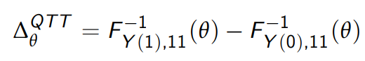
Armed  with this notation, we can formally define the QTT, which is difference between the inverse of F_Y(1),11 at quantile q and the inverse of the counterfactual distribution, F_Y(0),11. In LaTeX, this looks like

where I am using θ instead of q to denote the quantile. If your freaking out, just replace θ with the median and the above expression is simply the difference in the median outcome for the treatment units in period 1 with and without the treatment.

Given a random sample, the four distributions can all be estimated (nonparametrically) using the empirical cumulative distribution functions (ECDFs). Note, nonparametric and ECDF may be scary sounding, but these fancy words just mean plot the CDF of your data. No heavy lifting required. You can do this in Stata using -cumul- or -cdfplot-.

The counterfactual distribution, F_Y(0),11, cannot be directly observed in the data. So, estimation boils down to estimating the counterfactual CDF for the treatment units in period 1. In DID, estimation boils down to estimating the expected value of this counterfactual distribution. Here, we want to learn each of the quantiles of this distribution.

Fret not. In the DID setup, this is trivial. We examine how the average realized outcome changes over time for the control units and assume the average outcome for the treatment units would have evolved similarly. This allows us to estimate the counterfactual expected value for the treatment units in period 1 by simply adding this change to the average outcome for the treatment units in period 0. The ATT then follows as the difference between the average realized outcome for the treatment units in period 1 and this counterfactual expected value. 

There is no reason things can't be this trivial in the quantile context. We could examine how quantile q of the outcome changes over time for the control units and assume quantile q for the treatment units would have evolved similarly. This allows us to estimate the counterfactual quantile q for the treatment units in period 1 by simply adding this change to quantile q for the treatment units in period 0. The QTT at quantile q then follows as the difference between the outcome for the treatment units at quantile q in period 1 and this counterfactual value of quantile q. 

Easy, right? But, AI say this would be wrong!

This is where we need to listen to Bowie again and turn and face the strange. AI make the convincing argument that the estimator just described, which AI refer to as quantile difference-in-differences (QDID), relies on a set of inferior assumptions compared to an alternative estimator they refer to as quantile changes-in-changes (QCIC). Ahhhh, Bowie. 

While QCIC is strange at first glance, there are two important things to note. First, it is no more difficult to compute than QDID. Second, it makes sense intuitively once we think about it.

QCIC differs from QDID in only one way. QDID posits that quantile q of the Y(0) distribution for the treatment units would have evolved over time in an identical manner to quantile q of the Y(0) distribution for the control units. If you will, the parallel trends assumption holds at quantile q. Instead, QCIC is based on the assumption that quantile q of the Y(0) distribution for the treatment units would have evolved over time in an identical manner to quantile q' of the Y(0) distribution for the control units, where q' may not equal q. In other words, quantile q for the treatment units would have followed a parallel trend to quantile q' for the control units. That's it. That's the difference.

But, which quantile q' should we use? AI suggest we use the quantile q' associated with value of the outcome at quantile q for the treatment units in period 0. 

An illustration will make this clear. Returning to the job training example from above, suppose we are interested in estimating the QTT at the median. The sample median wage for the treatment units in period 0 is, say, $10/hr. So, we then turn to the wage distribution for the control units in period 0 and we see to which quantile $10/hr corresponds. If the treatment group is positively selected, $10/hr might represent, say, the 70th quantile of the wage distribution in period 0 for the control units. We then examine how the 70th quantile of the wage distribution changes over time for the control units and assume the median wage for the treatment units would have evolved similarly. If the 70th quantile for the control units increases to, say $12/hr in period 1, then the counterfactual median wage for the treatment units in period 1 is $12/hr. The QCIC estimate of the QTT at the median is then given by the realized median wage of the treatment units in period 1 minus $12/hr.  

A bit strange, indeed, but in hindsight it seems obvious. While we are assuming parallel trends between the treatment and control units across different quantiles, we are assuming parallel trends between treatment and control units with the same value of the outcome in the pretreatment period.

In contrast, QDID assumes parallel trends holds between treatment and control units at the same quantile, but potentially radically different values of the outcome in the pretreatment period. Since the quantile itself likely has no economic effect, it is much more likely that units with identical outcomes would follow a parallel trend in the absence of treatment, rather than units at identical quantiles. Finding a quantile's doppelgänger at a different quantile reminds me of another unlikely duo that were nevertheless a perfect match.

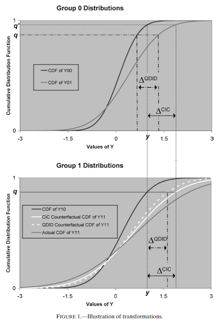
If you want to see AI's estimator in action, here is the picture that compares QDID and QCIC. It takes a while to process and I won't walk you through it here (since this post is already too long!), but if you sit with it, I promise it will make sense.

Formally, the estimator is written as follows.

It looks messy, but it is just a function of basic statistics! And, once again, Stata to the rescue. The command -cic- is available. There actually appear to be two versions floating around by different authors. The version by Blaise Melly is based on Melly & Santangelo (2015) and allows one to also control for covariates in the model. Their code is available here.

This post started by referencing Google Scholar. I will end that way as well. Citations of AI (while not too shabby) are dwarfed by citations to DID, and seem to be primarily by other econometric theory papers. In my view, not only does AI's approach provide a more complete analysis of the treatment, but it offers a way to distinguish yourself from the crowd.

As Bowie said, it's all about the changes. Perhaps we will see a change in the usage of AI in applied research moving forward. Perhaps there will even someday be a paper by Pedro Sant'Anna and Brant Callaway about staggered QCIC. 

UPDATE (5.16.2020)

Thanks to Wei Yang Tham for pointing out that AI is also available in the -qtte- package in R here.

Thanks also to Vitor Possebom (who must spend all his time reading!) for pointing out a related paper by Bonhomme & Sauder (2011). Of course, it makes use of imaginary numbers and I have strict rules against relying on made-up math. As I said above, I have issues.

References

Athey, S. and G.W. Imbens (2006), "Identification and Inference in Nonlinear Difference-In-Differences Models," Econometrica, 74, 431-497

Bonhomme, S. and U. Sauder (2011), "Recovering Distributions in Difference-in-Differences Models: A Comparison of Selective and Comprehensive Schooling," Review of Economics and Statistics, 93(2), 479-494

Melly, B. and G. Santangelo (2015), "The Changes-in-Changes Model with Covariates," unpublished manuscript.