Where the Magic Happens
It's been a difficult few weeks for all of us. But, it has been difficult for many for much longer than that. Many of us are finding it hard to focus on work, too busy wondering what we can do to help and often coming up (relatively) empty. For some, one's research may speak directly to aspects of the issues currently dominating the news. For many others, one's research may seem far less relevant to the current crisis.
That said, regardless of what the subject of your research is, if you are reading this blog it is because your research is largely empirical in nature. And, if it is empirical in nature, I am a firm believer your research can help depending on how you conduct your research.
I am not even remotely an expert, or even particularly well-informed, about all that ails our society. However, at the most simplistic level, I imagine it is fair to say that our problems relate to deep historical divides between the privileged and the under-privileged, between the rich and the poor, between those with power and those without, between those with lighter skin tones and those with darker skin tones, between so-called natives and immigrants. Fundamentally, our issues are about inequality and disparities in all forms.

The occasional use of interactions notwithstanding, it seems that the popularity of the potential outcomes framework really pushed us beyond the notion of constant marginal effects and brought a recognition of heterogeneous treatment effects across all agents. Despite this recognition, however, early work focused heavily on estimating the average treatment effect (ATE) in the population, or perhaps the average treatment effect on the treated (ATT). Thus, all that heterogeneity was relegated to the background.

Today, the focus on the ATE or ATT continues to dominate. That said, strides have been made to explore heterogeneity along certain dimensions in many studies. This is still typically done by splitting the sample into different demographic groups or by adding interactions in linear regression models. Regardless, this approach is fairly ad hoc, and perhaps an afterthought simply to appease referees.

In my opinion, one way that all empirical researchers can improve and can contribute to the current crises (plural) is to make distributional heterogeneity more front and center in our work. I have already discussed some ways this can happen in prior posts.

First, I wrote about the fallacy of the 'average man' here. In non-linear models, where marginal effects are observation-specific even if parameters are constant in the population, this might translate into spending more time analyzing and discussing the distribution of the marginal effects.
Second, I wrote about the Athey & Imbens (2006) changes-in-changes estimator here. Given the incredible popularity of difference-in-difference (DID) models, which are known to recover the ATT if all goes well, we could instead spend time recovering the full distribution of quantile treatment effects. A recent paper I neglected to mention earlier by Callaway & Li (2019) also extends the basic DID models to recover quantile treatment effects on treated. And, Callaway & Li provide code in the R package -qte-.
But, there are even more methods available for applied researchers to examine distributional effects of treatments. Amidst the chaos, I was reminded of this thanks to a new IZA Discussion Paper by Firpo et al. (2020). However, to place this paper in its proper context, let us revisit a literature that has remained for far too long on the fringes of applied work.
In the early 2000s, Barrett & Donald (2003) and Linton et al. (2005) made great strides in developing econometric tests for stochastic dominance (SD). If your training was like mine, you might have vaguely heard about SD in micro theory, not econometrics. But, SD is a very powerful concept. Since many may not recall, let us review.

Let F and G represent two different cumulative distribution functions (CDFs) of a random variable, Y, such as income. A social planner is deciding which distribution, F or G, is preferred. The planner's welfare function is given by
under distribution F and
W(G) = ∫v(y)dG(y)
under distribution G, where v(y) is the value function associated with a particular value, y. In other words, W(F) is the welfare the planner derives from the income distribution F given that the planner values each agent's individual income, y, using the value function v(y). Similarly for W(G).
Well, rather than computing W(F) and W(G) for all possible choices of the value function, v(y), or a single ad hoc choice of a value function, stochastic dominance can potentially simplify the comparison. We say that the distribution F first order stochastic dominates (FSD) the distribution G if W(F) ≥ W(G) for all value functions that are weakly increasing (i.e. v'(y) ≥ 0). Thus, if we know that F FSD G, then we know that any planner that (weakly) values more income to less would prefer distribution F regardless of the specific value function being used.
In practice, F FSD G if F lies on top of and/or to the right of G.

We describe FSD as a situation where the CDFs may kiss but they cannot cross.

FSD is a strong, powerful concept. Second order stochastic dominance is slightly weaker. We say that the distribution F second order stochastic dominates (SSD) the distribution G if W(F) ≥ W(G) for all value functions that are weakly increasing and concave (i.e. v'(y) ≥ 0, v''(y) ≤ 0).
In this case, if F SSD G, then we know that any planner that (weakly) values more income to less, but at a (weakly) decreasing rate, would prefer distribution F regardless of the specific value function being used. In practice, F SSD G if F initially lies on top of or to the right of G, but now they may cross at higher quantiles. Formally, SSD requires that the area under F is equal to or less than area under G at all values of y.

In this particular picture, SSD requires the area in (a) to be larger than the area in (b). This illustrates why SSD enables us to explore inequality and disparity in more detail as SSD let's us make strong statements about how one distribution compares to another accounting for the fact that we might value improvements more in the lower tail.
There are additional orders of SD (third and higher), but these are generally used only in finance as they become harder to interpret. There is also a theorem (somewhere) that two distributions can always be ranked according to stochastic dominance of some order.

Now, given the information learned by knowing that one distribution FSD or SSD another, the above mentioned papers develop statistical tests for such relationships. Such tests should be of interest to many, many applied researchers examining treatment effects because one can think of the two distributions, F and G, as corresponding to the distributions of potential outcomes.

Given a treatment, if we know, say, that the CDF of Y(1) SSD the CDF of Y(0), then we know that the treatment is preferred by any social planner that values the outcome at a weakly increasing and concave rate. That's powerful stuff! And, if we fail to find a first or second order stochastic relationship, then that too is telling since then we know that the treatment has important distributional consequences and different social planners -- all with seemingly reasonable value functions -- may disagree on the optimal course of action.
In fact, this is what I did in a few papers I wrote long ago. One looking at the effect of class size on student achievement and one looking at the male marriage premium. However, these papers are old and there are better methods to use today. For example, Donald & Hsu (2014) explicitly discuss testing for SD among potential outcomes distribution.

But, testing for stochastic dominance is not the only way we could better assess inequality and disparity in our applied research. Firpo & Pinto (2016) discuss other treatment effect parameters, beyond the ATE and ATT, that should be of greater interest to researchers. The authors term their parameters inequality treatment effects. They are defined as follows
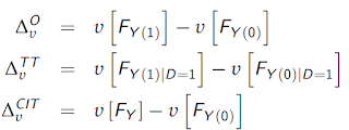
where υ[.] represents any inequality measure such as a Gini coefficient, interquartile range, Theil index, etc.
The first parameter is referred to as the overall inequality treatment effect and measures the difference in inequality between the two potential outcome distributions. The second parameter is the inequality treatment effect on the treated. The final parameter is the current inequality treatment effect and it compares the status quo distribution to the distribution in the absence of treatment. This is akin to the policy relevant treatment effect parameter of Heckman & Vytlacil (2001) as it compares the status quo distribution where agents have the decision to obtain a treatment or not to the counterfactual where the treatment does not exist.

Firpo & Pinto estimate these treatment effect parameters for a given choice of υ[.] under the conditional independence assumption by first estimating the distributions of the potential outcomes using inverse propensity score weighting. In light of recent events, improving our understanding of the effects of treatments and policies on the dispersion of economic outcomes seems like something to which we can all strive to contribute.

And, this brings us to this week, where a new working paper by Firpo et al. (2020) expands on this line of methods spanning nearly two decades. In this paper, the authors develop a new concept of stochastic dominance and then show how to apply it to the usual treatment effects setup. Their concept is called loss aversion-sensitive dominance (LASD).

Recall from above our comparison of two distributions, F and G, using the welfare functions
W(F) = ∫v(y)dF(y)
and
W(G) = ∫v(y)dG(y).
This paper differs from the above methods in two respects. First, the authors define the random variable, Y, as denoting changes in the outcomes of agents, not levels (i.e., changes from the pre-treatment to the post-treatment period). Second, the authors say that F LASD G if W(F) ≥ W(G) for all choices of the value function that satisfy three properties:
1. v(y) ≤ 0 for all y < 0, v(0) = 0, and v(y) ≥ 0 for all y > 0
2. v'(y) ≥ 0 for all y
3. v'(-y) ≥ v'(y) for all y > 0
Thus, the value function must value gains, abhor losses, weakly value higher gains, and exhibit loss aversion such that a reduction in losses is valued more than an equivalent increase in gains.
The authors derive tests of LASD and then illustrate the method by comparing the change in outcomes for individuals randomly assigned to two different treatment arms. This test allows the authors to understand whether one treatment arm unambiguously is preferred to the other when the social planner exhibits loss aversion.

At the risk of being too somber and too preachy, we can all make more of a contribution to alleviating some of society's ills, in my view, if we devote the time and effort to better understand the distributional consequences of whatever treatments or policies we study. We have too many wondrous tools at our disposal to be content to estimate averages and then investigate maybe a few ad hoc sources of heterogeneity. It's time to venture outside our comfort zone when it comes to econometric methods for the sake of making the world a better place.

References
Athey, S. and G.W. Imbens (2006), "Identification and Inference in Nonlinear Difference-In-Differences Models," Econometrica, 74, 431-497
Barrett, G.F. and S.G. Donald (2003), "Consistent Tests for Stochastic Dominance," Econometrica, 71(1), 71-104
Callaway, B. (2020), "Bounds on Distributional Treatment Effect Parameters using Panel Data with an Application on Job Displacement," Journal of Econometrics, forthcoming
Callaway, B. and T. Li (2019), "Quantile Treatment Effects in Difference in Differences Models with Panel Data," Quantitative Economics, 10(4), 1579-1618
Donald, S.G. and Y.C. Hsu (2014), "Estimation and Inference for Distribution Functions and Quantile Functions in Treatment Effect Models," Journal of Econometrics, 178, 383-397
Firpo, S., A.F. Galvao, M. Kobus, T. Parker, P. Rosa-Dias (2020), "Loss Aversion and the Welfare Ranking of Policy Interventions," IZA Discussion Paper No. 13176
Firpo, S. and C. Pinto (2016), "Identification and Estimation of Distributional Impacts of Interventions Using Changes in Inequality Measures," Journal of Applied Econometrics, 31(3), 457-486
Linton, O., E. Maasoumi, Y.J. Whang (2005), "Consistent Testing for Stochastic Dominance Under General Sampling Schemes," Review of Economic Studies, 72(3), 735-765


